BADA ARPM Descent Calculation

Example of BADA4 trajectory full descent taking into account the compelte BADA ARPM model

• 
• 
• 
• 

import matplotlib.pyplot as plt

from pyBADA import TCL as TCL
from pyBADA import myTypes
from pyBADA.badaAircraft import BadaAircraft

# load BADA specific model
AC = BadaAircraft(badaFamily="BADA4", badaVersion="DUMMY", acName="Dummy-TWIN")

trajectory = TCL.apcDescentCalculation(
    AC=AC,
    descentType=myTypes.DescentType.CASMACH,
    pressureAltitude=myTypes.PressureAltitude(
        initPressureAltitude=AC.hmo,
        finalPressureAltitude=0,
        stepPressureAltitude=1000,
    ),
    speed=myTypes.Speed(
        accelerationLevelKind=myTypes.AccelerationLevelKind.BEFORE,
        stepSpeed=10,
    ),
    mass=0.7 * AC.MTOW,
    meteo=myTypes.Meteo(deltaTemp=0),
    CASMACHProfileConfiguration=myTypes.DescentCASMACHProfileConfiguration(),
)


# ========================================================
# OUTPUT and PLOTS
# ========================================================

Hp = trajectory.getAllValues(AC, "Hp")
mass = trajectory.getAllValues(AC, "mass")
CAS = trajectory.getAllValues(AC, "CAS")
TAS = trajectory.getAllValues(AC, "TAS")
fuel = trajectory.getAllValues(AC, "FUEL")
fuelConsumed = trajectory.getAllValues(AC, "FUELCONSUMED")
time = trajectory.getAllValues(AC, "time")
dist = trajectory.getAllValues(AC, "dist")

# ---------------------------------------------------------
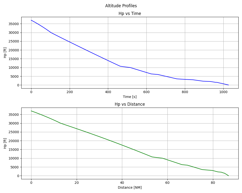
# Plot 1: Hp = f(time) and Hp = f(dist) as 2 subplots
# ---------------------------------------------------------
fig1, (ax1, ax2) = plt.subplots(2, 1, figsize=(10, 8))
fig1.suptitle("Altitude Profiles")

# Hp = f(time)
ax1.plot(time, Hp, color="blue")
ax1.set_title("Hp vs Time")
ax1.set_xlabel("Time [s]")
ax1.set_ylabel("Hp [ft]")
ax1.grid(True)

# Hp = f(dist)
ax2.plot(dist, Hp, color="green")
ax2.set_title("Hp vs Distance")
ax2.set_xlabel("Distance [NM]")
ax2.set_ylabel("Hp [ft]")
ax2.grid(True)

plt.tight_layout()

# ---------------------------------------------------------
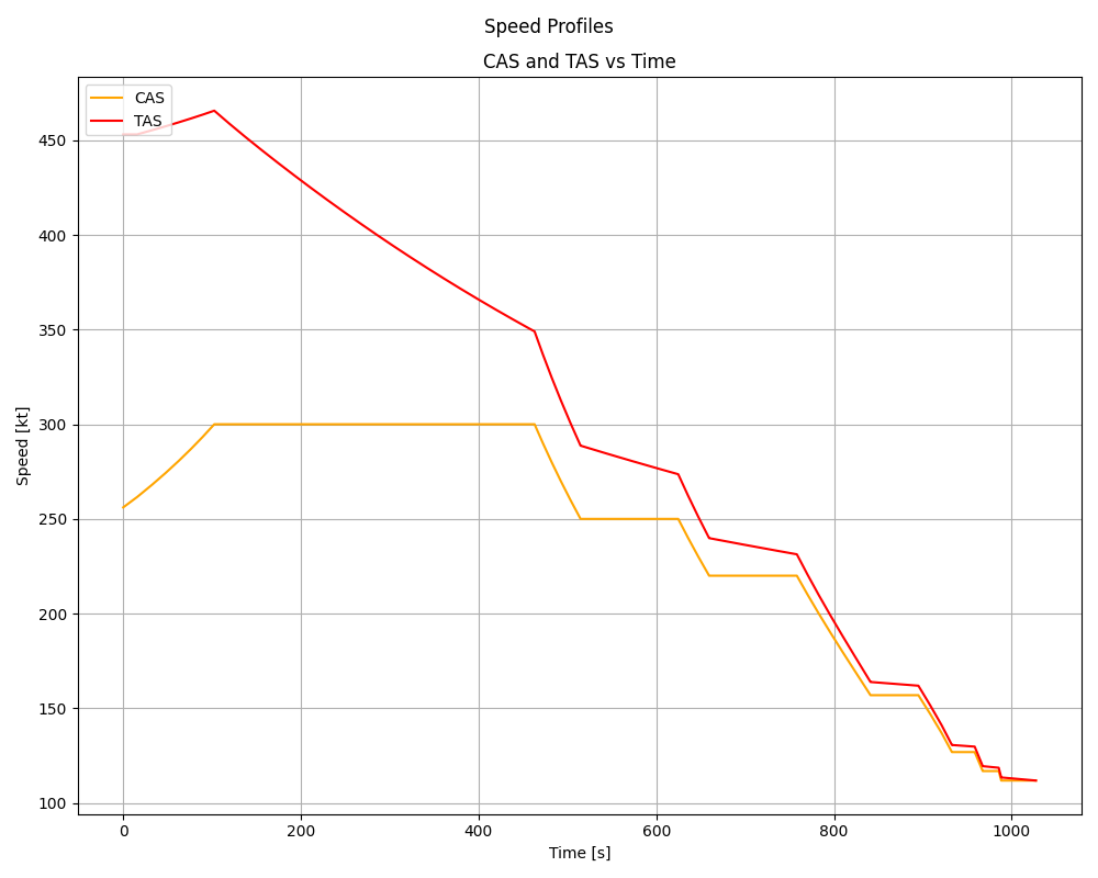
# Plot 2: CAS = f(time) and TAS = f(time) on a single axis
# ---------------------------------------------------------
fig2, ax3 = plt.subplots(figsize=(10, 8))
fig2.suptitle("Speed Profiles")

# Plot both CAS and TAS on the same axes
ax3.plot(time, CAS, color="orange", label="CAS")
ax3.plot(time, TAS, color="red", label="TAS")

# Single set of labels and grid
ax3.set_title("CAS and TAS vs Time")
ax3.set_xlabel("Time [s]")
ax3.set_ylabel("Speed [kt]")
ax3.grid(True)
ax3.legend(loc="upper left")

plt.tight_layout()

# ---------------------------------------------------------
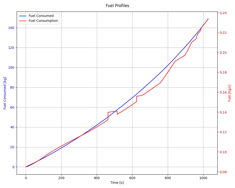
# Plot 3: fuelConsumed = f(time) and fuel = f(time)
# ---------------------------------------------------------
fig3, ax5 = plt.subplots(figsize=(10, 8))
fig3.suptitle("Fuel Profiles")

# Primary Y-axis (Left): fuelConsumed = f(time)
color_consumed = "blue"
ax5.plot(time, fuelConsumed, color=color_consumed, label="Fuel Consumed")
ax5.set_xlabel("Time [s]")
ax5.set_ylabel("Fuel Consumed [kg]", color=color_consumed)
ax5.tick_params(axis="y", labelcolor=color_consumed)
ax5.grid(True)

# Secondary Y-axis (Right): fuel = f(time)
ax6 = ax5.twinx()  # Create a second axes that shares the same x-axis
color_rate = "red"
ax6.plot(time, fuel, color=color_rate, label="Fuel Consumption")
ax6.set_ylabel("Fuel [kg/s]", color=color_rate)
ax6.tick_params(axis="y", labelcolor=color_rate)

# Combine legends from both axes so they appear in one box
lines_1, labels_1 = ax5.get_legend_handles_labels()
lines_2, labels_2 = ax6.get_legend_handles_labels()
ax5.legend(lines_1 + lines_2, labels_1 + labels_2, loc="upper left")

plt.tight_layout()

# ---------------------------------------------------------
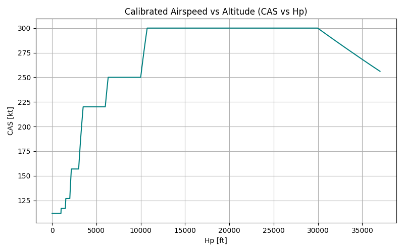
# Plot 4: CAS = f(Hp)
# ---------------------------------------------------------
fig4, ax7 = plt.subplots(figsize=(8, 5))

# CAS = f(Hp)
ax7.plot(Hp, CAS, color="teal")
ax7.set_title("Calibrated Airspeed vs Altitude (CAS vs Hp)")
ax7.set_xlabel("Hp [ft]")
ax7.set_ylabel("CAS [kt]")
ax7.grid(True)

plt.tight_layout()

# Display all the figures
plt.show()